Tutorial
First steps
Installing GAMtools
The first step in the GAMtools tutorial is to make sure that GAMtools
is properly installed. Try to run gamtools --help and make sure that you
get the following ouput:
$ gamtools --help
usage: gamtools [-h]
              {call_windows,convert,enrichment,matrix,permute_segregation,plot_np,process_nps,select}
              ...
If this command gives you an error message, it is likely that GAMtools has not been installed correctly. Please ensure you have followed the steps outlined in the Installation guide.
Downloading the tutorial data
Once GAMtools is working correctly, you need to download some example data
to work with during the tutorial. The tutorial data is located on the GAMtools
website. Download the tutorial data
(e.g. by using wget), extract it and cd into the newly created directory. The
directory should contain a folder called fastqs and a file called
clean.sh.
$ wget http://gam.tools/tutorial_data.tar.gz
$ tar zxvf tutorial_data.tar.gz
$ cd gamtools_tutorial
$ ls
clean.sh  fastqs/
The fastqs folder contains sequencing data from 100 separate nuclear
profiles (NPs):
$ ls fastqs/
NP_001.fq.gz  NP_026.fq.gz  NP_051.fq.gz  NP_076.fq.gz
NP_002.fq.gz  NP_027.fq.gz  NP_052.fq.gz  NP_077.fq.gz
NP_003.fq.gz  NP_028.fq.gz  NP_053.fq.gz  NP_078.fq.gz
NP_004.fq.gz  NP_029.fq.gz  NP_054.fq.gz  NP_079.fq.gz
NP_005.fq.gz  NP_030.fq.gz  NP_055.fq.gz  NP_080.fq.gz
...
NP_025.fq.gz  NP_050.fq.gz  NP_075.fq.gz  NP_100.fq.gz
These files are the primary raw output of a GAM experiment. The first thing we need to do with the sequencing data is to “map” it to a genome. The example data comes from mouse embryonic stem cells, so we need to map it to the mouse genome, which we will do using bowtie2. If you already have bowtie2 and a mouse genome assembly installed and configured on your local machine, you can skip the next step (mouse assembly mm9 is preferred, but any other assembly should work with this tutorial).
Configuring bowtie2
If you have not yet installed bowtie2, please follow the installation instructions on the bowtie2 homepage. Once you have bowtie installed, verify that everything is working correctly:
$ bowtie2 --version
/home/rob_000/bowtie2-2.2.9/bowtie2-align-s version 2.2.9
64-bit
Built on Windows8
30 Apr 2016 18:13:39
We next need to provide the sequence of the mouse genome for bowtie to map against. If you wish, you can download and configure the full mouse mm9 “index” from Illumina. However, the 100 sequencing datasets provided as part of the tutorial only contain sequencing data from a small region of chromosome 19, so you can also use a special truncated index containing only the sequence of mouse chromosome 19. This will allow bowtie to run much faster whilst using less RAM, and is perfectly sufficient for completing this tutorial. If you wish to use the tutorial index, download it from the GAMtools website, extract it to the same folder as fastqs and configure bowtie to use the new truncated index:
$ wget http://gam.tools/tutorial_index.tar.gz
$ tar zxvf tutorial_index.tar.gz
$ ls
clean.sh fastqs/ genome/
$ export BOWTIE2_INDEXES=$(pwd)/genome/
$ ls $BOWTIE2_INDEXES
genome.1.bt2  genome.3.bt2  genome.rev.1.bt2  chr19.size
genome.2.bt2  genome.4.bt2  genome.rev.2.bt2
Mapping the sequencing data and calling positive windows
The GAMtools command used for mapping NP sequencing data is gamtools
process_nps. The process_nps command has a lot of different parameters
and options, you can use the --help flag to get a full description of all
the available parameters. Further information about the process_nps
command can also be found on the process_nps page.
$ gamtools process_nps --help
usage: gamtools process_nps [-h] -g GENOME_FILE [-o OUPUT_DIRECTORY]
                            [-f FITTINGS_DIRECTORY] [-d DETAILS_FILE] [-i]
                            [-b] [-c] [-w WINDOW_SIZE [WINDOW_SIZE ...]] [-m]
                            [-s MATRIX_SIZE [MATRIX_SIZE ...]]
                            [--qc-window-size QC_WINDOW_SIZE]
                            [--additional-qc-files [ADDITIONAL_QC_FILES [ADDITIONAL_QC_FILES ...]]]
                            [-q MINIMUM_MAPQ] [--doit-db-file DEP_FILE]
                            [--doit-backend {sqlite3,json,dbm}]
                            [--doit-verbosity {0,1,2}]
                            [--doit-reporter {json,console,zero,executed-only}]
                            [--doit-process NUM_PROCESS]
                            [--doit-parallel-type {process,thread}]
                            INPUT_FASTQ [INPUT_FASTQ ...]
For now, we can just use the default options. That means that all we need to specifiy
is a genome file (using -g/--genome-file) and a list of input fastq files:
$ gamtools process_nps -g genome/chr19.size fastqs/*.fq.gz
This tells GAMtools to use the genome file genome/chr19.size .You
will have this file if you downloaded the special truncated index. If you
are using your own mouse genome index, you will have to specify your own
genome file (which is usually named something like mm9.chrom.sizes).
The next argument tells GAMtools to process all of the files with the
extension “.fq.gz” in the folder called “fastqs”. When you run the
command, GAMtools will start mapping the sequencing data, and you
should see an output like this:
$ gamtools process_nps -g genome/chr19.size fastqs/*.fq.gz
-- Creating output directory
.  Mapping fastq:fastqs/NP_025.fq.gz
.  Mapping fastq:fastqs/NP_017.fq.gz
.  Mapping fastq:fastqs/NP_065.fq.gz
.  Mapping fastq:fastqs/NP_014.fq.gz
.  Mapping fastq:fastqs/NP_090.fq.gz
.  Mapping fastq:fastqs/NP_078.fq.gz
GAMtools will then proceed to map all 100 individual sequencing files to the mouse genome. This will take around 5 minutes if you are using the truncated index and a moderately fast computer. If you are using your own full mouse genome index, it may take a little longer. Once it has mapped the files, GAMtools will sort the mapped files, remove PCR duplicates and create an index for fast data retrieval.
The final steps are to compute the number of
reads from each NP that overlap each 50kb window in the supplied genome file,
and then to use this read coverage count to determine which of the windows was
present in the original NP. After performing this “window calling” step,
gamtools produces a file called segregation_at_50kb.table. This file
contains one row per 50kb window, and one column per NP:
# Show the first 10 rows and first 5 columns of the segregation table
$ head segregation_at_50kb.table | cut -f 1-5
chrom   start   stop    fastqs/NP_027.rmdup.bam       fastqs/NP_020.rmdup.bam
chr19   0       50000   0       0
chr19   50000   100000  0       0
chr19   100000  150000  0       0
chr19   150000  200000  0       0
chr19   200000  250000  0       0
chr19   250000  300000  0       0
chr19   300000  350000  0       0
chr19   350000  400000  0       0
chr19   400000  450000  0       0
For each NP column, 0 indicates that the window was not present in the NP,
whereas 1 indicates that the window was present. This table is the crucial
and most important output of a GAM experiment - all further downstream
analysis will generally be based on the segregation table.
Producing proximity matrices
Now that we have produced a segregation table at 50kb resolution, we can
use it to calculate a proximity matrix, using the gamtools matrix
command. As for the process_nps command, the matrix command has
a lot of different options, which can be explored further using
the --help flag or on the gamtools matrix page.
$ gamtools matrix --help
usage: gamtools matrix [-h] -r REGION [REGION ...] -s SEGREGATION_FILE
                       [-f {csv.gz,txt,csv,txt.gz,npz}]
                       [-t {cosegregation,linkage,dprime}] [-o OUTPUT_FILE]

optional arguments:
  -h, --help            show this help message and exit
  -r REGION [REGION ...], --regions REGION [REGION ...]
                        Specific genomic regions to calculate matrices for. If
                        one region is specified, a matrix is calculated for
                        that region against itself. If more than one region is
                        specified, a matrix is calculated for each region
                        against the other. Regions are specified using UCSC
                        browser syntax, i.e. "chr4" for the whole of
                        chromosome 4 or "chr4:100000-200000" for a sub-region
                        of the chromosome.
  -s SEGREGATION_FILE, --segregation_file SEGREGATION_FILE
                        A segregation file to use as input
  -f {csv.gz,txt,csv,txt.gz,npz}, --output-format {csv.gz,txt,csv,txt.gz,npz}
                        Output matrix file format (choose from: csv.gz, txt,
                        csv, txt.gz, npz, default is txt.gz)
  -t {cosegregation,linkage,dprime}, --matrix-type {cosegregation,linkage,dprime}
                        Method used to calculate the interaction matrix
                        (choose from: cosegregation, linkage, dprime, default
                        is dprime)
  -o OUTPUT_FILE, --output-file OUTPUT_FILE
                        Output matrix file. If not specified, new file will
                        have the same name as the segregation file and an
                        extension indicating the genomic region(s) and the
                        matrix method
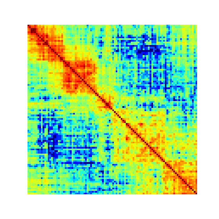
We can start by asking for the proximity matrix for our region of interest in png format:
$ gamtools matrix -s segregation_at_50kb.table \
> -r chr19:10,000,000-15,000,000 -o my_matrix.png
starting calculation for chr19:10,000,000-15,000,000
region size is: 100 x 100 Calculation took 1.05s
Saving matrix to file my_matrix.png
Done!
$ open my_matrix.png
You should see an image file that looks like this:
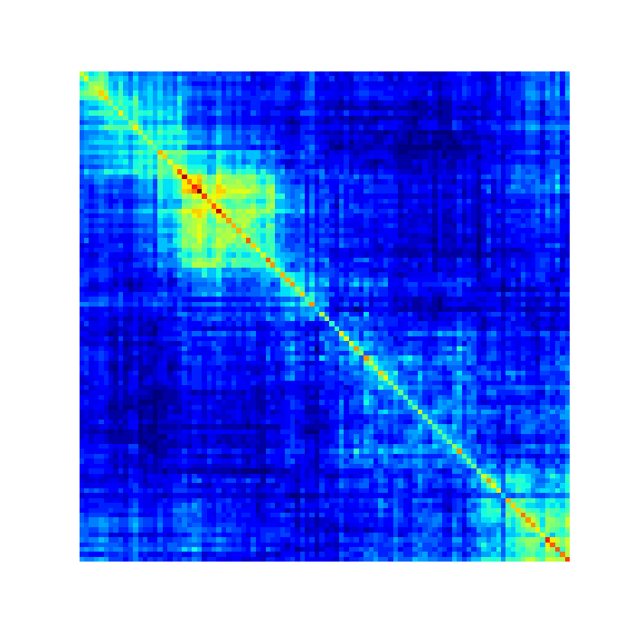
Note that the example data for this tutorial only covers this specific region of chromosome 19, so if you specify a larger or different region you will get some strange looking results:
$ gamtools matrix -s segregation_at_50kb.table \
> -r chr19:8,000,000-17,000,000 -o larger_matrix.png
starting calculation for chr19:8,000,000-17,000,000
region size is: 180 x 180 Calculation took 3.47s
Saving matrix to file larger_matrix.png
Done!
$ open larger_matrix.png
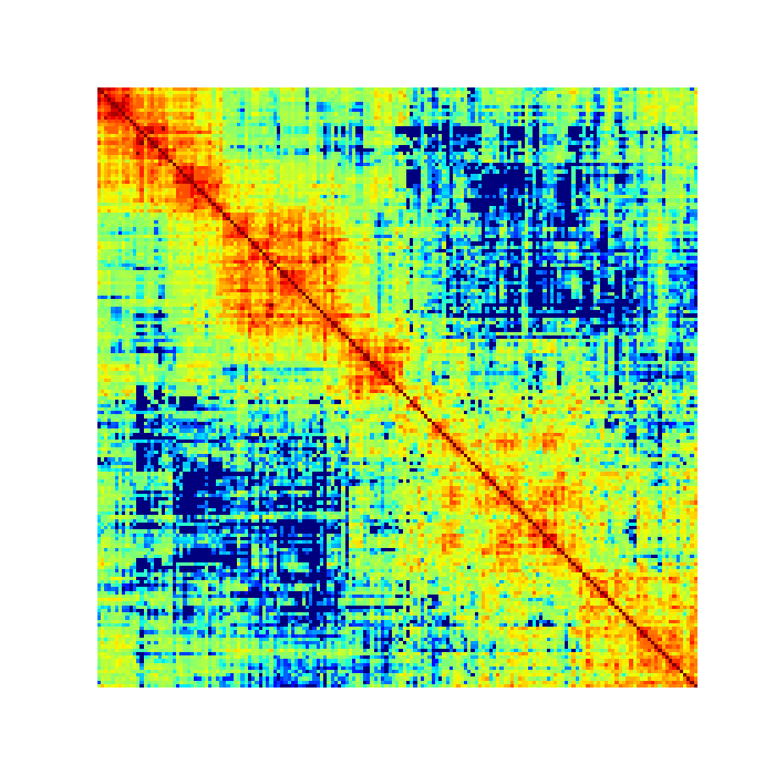
By default, GAMtools produces proximity matrices using the
normalized linkage disequilibrium (or D’). In this case, it first
calculates how many times each pair of windows are found together in
the same NP, and then normalizes the matrix according to how many times
each window is detected across the collection of NPs. You can create
raw, un-normalized co-segregation matrices by specifying the
cosegregation option using the -t/--matrix-type flag:
$ gamtools matrix -s segregation_at_50kb.table \
> -r chr19:10,000,000-15,000,000 -o cosegregation_matrix.png \
> -t cosegregation
starting calculation for chr19:10,000,000-15,000,000
region size is: 100 x 100 Calculation took 1.05s
Saving matrix to file cosegregation_matrix.png
Done!
$ open cosegregation_matrix.png
Working at different resolutions
If we want to produce a proximity matrix at a resolution other than
50kb, we first need to calculate a segregation table at that
resolution. We can generate another segregation table using the
process_nps command, specifying the resolution using the
-w/--window-sizes flag. For example at 30kb resolution:
$ gamtools process_nps -w 30000 -g genome/chr19.size fastqs/*.fq.gz
-- Creating output directory
-- Mapping fastq:fastqs/NP_025.fq.gz
-- Mapping fastq:fastqs/NP_017.fq.gz
-- Mapping fastq:fastqs/NP_065.fq.gz
-- Mapping fastq:fastqs/NP_014.fq.gz
-- Mapping fastq:fastqs/NP_090.fq.gz
-- Mapping fastq:fastqs/NP_078.fq.gz
...
...
...
.  Getting coverage:30kb windows
.  Calling positive windows:30kb
Notice that all the lines except the last two begin with --, whereas the
last two lines begin with .. The -- indicates that GAMtools
realized that these tasks have already been completed and therefore do not
need to be re-run. When we re-calculate a segregation table at a new
resolution, we don’t need to remap all the individual fastq files, we only
need to re-compute the read depth over all 30kb windows, and then decide
which 30kb windows were positive in each NP.
To create proximity matrices at the new resolution, we need to specify
the new segregation table: segregation_at_30kb.table.
$ gamtools matrix -s segregation_at_30kb.table \
> -r chr19:10,000,000-15,000,000 -o 30kb_matrix.png
starting calculation for chr19:10,000,000-15,000,000
region size is: 167 x 167 Calculation took 0.047s
Saving matrix to file 30kb_matrix.png
Done!
$ open 30kb_matrix.png
Performing quality control checks
If you are generating your own GAM datasets, you will want to perform some
checks to ensure your NPs are of sufficient quality. GAMtools will
generate a table of QC parameters automatically for each NP if you use
the process_nps command with the -c/--do-qc flag.
Note
Performing quality control requires a number of additional dependencies to be installed. Please ensure that gamtools test runs with no errors before continuing with this section.
Re-running the gamtools process_nps command with the --do-qc flag
will instruct GAMtools to run a number of additional tasks. Your
output should look something like this:
$ gamtools process_nps --do-qc -g genome/chr19.size fastqs/*.fq.gz
-- Creating output directory
-- Mapping fastq:fastqs/NP_025.fq.gz
-- Mapping fastq:fastqs/NP_017.fq.gz
-- Mapping fastq:fastqs/NP_065.fq.gz
...
...
...
.  Creating QC parameters file with default values
.  Getting mapping stats
.  Getting segregation stats
.  Running fastqc:fastqs/NP_042.fq.gz
.  Running fastqc:fastqs/NP_043.fq.gz
...
.  Running fastqc:fastqs/NP_070.fq.gz
.  Running fastq_screen:fastqs/NP_063.fq.gz
.  Running fastq_screen:fastqs/NP_050.fq.gz
...
.  Running fastq_screen:fastqs/NP_081.fq.gz
.  Getting quality stats
.  Getting contamination stats
.  Merging stats files
.  Finding samples that pass QC
.  Filtering samples based on QC values:50kb
By default, GAMtools generates several QC files, each containing different information about the collection of NPs:
- The number of sequenced, mapped, and unique (i.e. excluding PCR duplicates) reads are saved in
mapping_stats.txt- Statistics regarding the number and distribution of positive windows are saved in
segregation_stats.txt- Statistics regarding the sequencing quality scores and the number of mono- and di-nucleotide repeat containing reads are calculated by fastqc and saved to
quality_stats.txt- Statistics regarding the percentage of reads mapping to different genomes (i.e. contaminating reads) are calculated by fastq_screen and saved to
contamination_stats.txt- These statistics files are merged together and the resulting table containing all the different QC parameters is saved to
merged_stats.txt
Once the merged stats table has been saved, GAMtools will
attempt to filter out “poor quality” NPs, and generates a file
called samples_passing_qc.txt containing only high-quality
NPs. GAMtools filters out NPs which match any rules in the
qc_parameters.cfg file, which is created with some default
rules if it does not exist. Finally, GAMtools creates new
segregation tables that exclude poor-quality NPs. In our case,
this file will be called segregation_at_50kb.passed_qc.table.
You can use this new segregation table to re-generate the
proximity matrices (see Producing proximity matrices).